How Hopfield Networks are a special case of the biologically plausible Sparse Distributed Memory.

Going off citation count for their original, seminal papers, Hopfield Networks are ~24x more popular than Sparse Distributed Memory (SDM) (24,362 citations versus 1,337). I think this is a shame because SDM can not only be viewed as a generalization of both the original and more modern Hopfield Networks but also passes a higher bar for biological plausbility – having a one-to-one mapping to the circuitry of the cerebellum. Additionally, like Hopfield Networks, SDM has been shown to closely relate to the powerful Transformer deep learning architecture.

In this blog post, we first provide background on Hopfield Networks. We then review how Sparse Distributed Memory (SDM) is a more general form of the original Hopfield Network. Finally, we provide insight into how modern improvements to the Hopfield Network modify the weighting of patterns, making them even more convergent with SDM. (In other words, SDM can be seen as pre-empting modern Hopfield Net innovations).

Summary of how modifications to SDM and Hopfield Networks relate them to Transformers and the Brain. Question marks denote uncertain but potential links.

Background on SDM and Hopfield Networks

The fundamental difference between SDM and Hopfield Networks lies in the primitives they use. In SDM, the core primitive is neurons that patterns are written into and read from. Hopfield Networks do a figure-ground inversion, where the core primitive is patterns and it is from their storage/retrieval that neurons implicitly appear.

To make this more concrete, we first provide a quick background on how SDM works:

SDM Background

If you like videos then watch the first 10 mins of this talk I gave on how SDM works and skip the rest of this section.

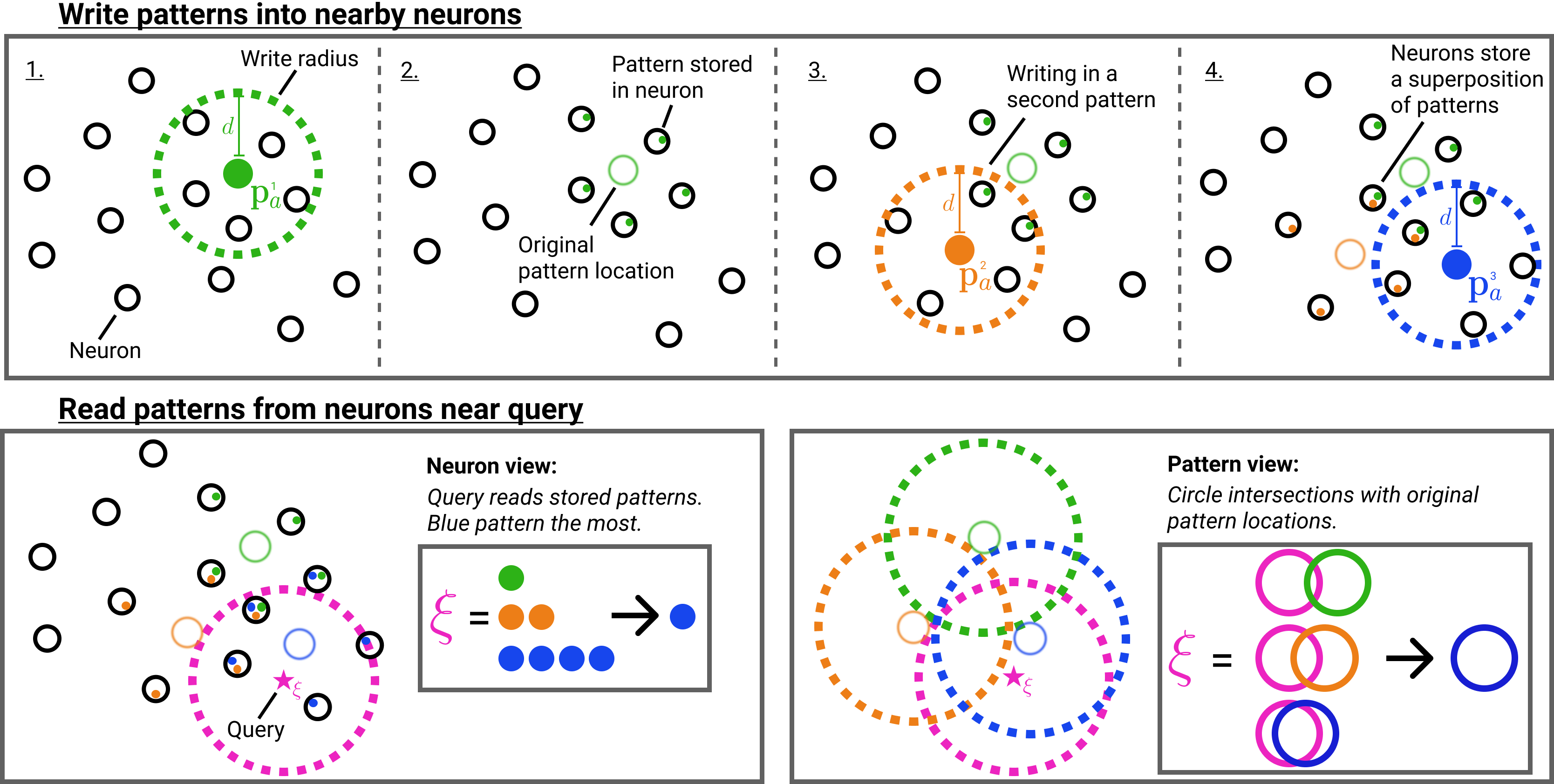
Summary SDM write operations (top row) and read operations (bottom row). The bottom left sub-figure shows the neuron view. The bottom right sub-figure shows how the neurons can be abstracted away and the original pattern locations considered.

To keep things simple, we will introduce the continuous version of SDM, where all neurons and patterns exist on the \(L^2\) unit norm hypersphere and cosine similarity is our distance metric. The original version of SDM used binary vectors and the Hamming distance metric.

SDM randomly initializes the addresses of \(r\) neurons on the \(L^2\) unit hypersphere in an \(n\) dimensional space. These neurons have addresses that each occupy a column in our address matrix \(X_a \in (L^2)^{n\times r}\), where \(L^2\) is shorthand for all \(n\)-dimensional vectors existing on the \(L^2\) unit norm hypersphere. Each neuron also has a storage vector used to store patterns represented in the matrix \(X_v \in \mathbb{R}^{o\times r}\), where \(o\) is the output dimension.

Patterns also have addresses constrained on the \(n\)-dimensional \(L^2\) hypersphere that are determined by their encoding; pattern encodings can be as simple as flattening an image into a vector or as complex as preprocessing the image through a deep convolutional network.

Patterns are stored by activating all nearby neurons within a cosine similarity threshold \(c\), and performing an elementwise summation with the activated neurons’ storage vector. Depending on the task at hand, patterns write themselves into the storage vector (e.g., during a reconstruction task) or write another pattern, possibly of different dimension (e.g., writing in their one hot label for a classification task).

Because in most cases we have fewer neurons than patterns, the same neuron will be activated by multiple different patterns. This is handled by storing the pattern values in superposition via the aforementioned elementwise summation operation. The fidelity of each pattern stored in this superposition is a function of the vector orthogonality and dimensionality \(n\).

Using \(m\) to denote the number of patterns, matrix \(P_a \in (L^2)^{n\times m}\) for the pattern addresses, and matrix \(P_v \in \mathbb{R}^{o\times m}\) for values the patterns want to write, the SDM write operation is: \begin{align} \label{eq:SDMWriteMatrix} X_v = P_v b_c \big ( P_a^T X_a \big ), \qquad b_c(e)= \begin{cases} 1, & \text{if}\ e \geq c
& \text{else} \; 0, \end{cases} \end{align} where \(b(e)\) performs an element-wise binarization of its input to determine which pattern and neuron addresses are within the cosine similarity threshold \(c\) of each other.

Having written patterns into our neurons, we read from the system by inputting a query \(\boldsymbol{\xi}\), that again activates nearby neurons. Each activated neuron outputs its storage vector and they are all summed elementwise to give a final output \(\mathbf{y}\). The output \(\mathbf{y}\) can be interpreted as an updated query and optionally \(L^2\) normalized again as a post processing step:

\begin{align} \label{eq:SDMReadMatrix} \mathbf{y} = X_v b_c \big ( X_a^T \boldsymbol{\xi} \big). \end{align}

Intuitively, SDM’s query will update towards the values of the patterns with the closest addresses. This is because the patterns with the closest addresses will have written their values into more neurons that the query reads from than any competing patterns. For example, in the summary figure above, the blue pattern address is the closest to the query meaning that it appears the most in those nearby neurons the query reads from.

Another potentially useful perspective is to see SDM as a single hidden layer MLP with a few modifications:

• All neuron addresses \(X_a\) are randomly initialized and fixed.
• All \(X_a\), \(P_a\) patterns and \(\boldsymbol{\xi}\) queries are \(L^2\) normalized.
• Only neurons above the activation threshold remain on so the activation function is not piecewise. They also use a Heaviside step function being 0 or 1 (this is not differentiable).
• The neurons have no bias term.

In a recent paper, we resolve a number of these modifications to make SDM more compatible with Deep Learning. This results in a model that is very good at continual learning!

How our SDM notation can be mapped onto the structure of a single hidden layer MLP.

In another paper, we show that the SDM update rule is closely approximated by the softmax update rule used by Transformer Attention. This will be relevant later with newer versions of Hopfield Networks that also show this relationship.

Hopfield Background

Hopfield Networks before the modern continuous version all use bipolar vectors \(\bar{\mathbf{a}} \in \{-1,1\}^n\) where the bar denotes bipolarity. The Hopfield Network update rule in matrix form, in its typical auto-associative format where \(P_v=P_a\) is:¹

\begin{equation} \label{eq:HopfieldUpdateRule} \bar{\mathbf{y}} = \bar{g}( \bar{P}_a \bar{P}_a^T \bar{\boldsymbol{\xi}} ) \qquad \bar{g}(e)= \begin{cases} 1, & \text{if}\ e> 0
, & \text{else} \; -1, \end{cases} \end{equation}

Interpreting this equation from the perspective of SDM, we first compute a re-scaled and approximate version of the cosine similarity between the query and pattern addresses \(\bar{P}_a^T \bar{\boldsymbol{\xi}}\). This can be done by taking a dot product between bipolar vectors and dividing by \(n\) to convert the interval our bipolar values can take from [-\(n\), \(n\)] to [-1,1] of cosine similarity:

\begin{equation} \label{eq:BipolarHammConversion} \mathbf{x}^T \mathbf{y} \approx \frac{\bar{\mathbf{x}}^T\bar{\mathbf{y}}}{n} \end{equation}

This relationship is exact with binary SDM and bipolar Hopfield but we leave this relationship to the Appendix B.6 of our paper.

We use this distance metric to weight each pattern before mapping back into our bipolar space with \(\bar{g}(\cdot)\).

Instead of first multiplying the query with the pattern addresses (\(\bar{P}_a^T \bar{\boldsymbol{\xi}}\)) like in SDM, Hopfield Networks instead typically perform \(\bar{P}_a \bar{P}_a^T=M\) which gives us a symmetric, \(n \times n\) dimensional matrix. We can interpret this symmetric matrix \(M\) as containing \(n\) neurons where each neuron’s address is a row and its value vector is the corresponding column, which by symmetry is the row transpose. Therefore, the number of neurons is defined by the pattern dimensionality \(n\) and the neuron address and value vectors are derived from \(\bar{P}_a \bar{P}_a^T\). This is how neurons emerge from the patterns in Hopfield Networks.

What is most distinct about this operation in comparison with SDM is that there is no activation threshold between the patterns and query (\(\bar{P}_a^T \bar{\boldsymbol{\xi}}\)). As a result, every pattern has an effect on the update rule including positive attraction and negative repulsion forces. We will see how more modern versions of the Hopfield Network have in fact re-implemented activation thresholds that are increasingly reminiscent of that used by SDM.

SDM as a Generalization of Hopfield Networks

It was first established by Keeler that SDM was a generalization of Hopfield Networks. Hopfield Networks can be represented by SDM’s neuron primitives as a special case where there are no distributed reading or writing operations. This makes the weighting of patterns in the read operation the bipolar re-scaling of the cosine similarity to the query.

The Hopfield version of SDM has neurons centered at each pattern so \(r=m\) and \(X_a=P_a\). Distributed writing and reading are removed by setting the cosine similarity threshold for writing to \(d_\text{write}=1\) and for reading to \(d_\text{read}=-1\).

This means patterns are only written to the neurons centered at them and the query reads from every neuron. In addition, for reading, rather than binary neuron activations using the Heaviside function \(b(\cdot)\), neurons are weighted by the bipolar version of the cosine similarity given by \(\bar{\mathbf{x}}^T\bar{\mathbf{y}}\). Writing out the SDM read operation in full with bipolar vectors that make our normalizing constant unnecessary, we have:

Looking first at the write operation where \(d_\text{write}=0\):

where \(I\) is the identity matrix and \(P_v=P_a\) in the typical autoassociative setting. For the read operation we remove the threshold and cosine similarity re-scaling:

Together, these modifications turn SDM using neuron representations into the original Hopfield Network:

Differences between SDM and Hopfield Networks

While Hopfield Networks have been traditionally presented and used in an autoassociative fashion, by using a synchronous update rule they can also be heteroassociative \(\bar{\mathbf{y}} = \bar{g}( \bar{P}_v \bar{P}_a^T \bar{\boldsymbol{\xi}} )\) but do not work as well. However, a solution is to operate autoassociatively but concatenate together the pattern address and pointer as was introduced here. However, this concatenation is less biologically plausible than SDMs solution that has separate input lines capable of carrying different key and value vectors.

A second and more important difference between SDM and Hopfield Networks is that the latter is biologically implausible because of the weight transport problem, whereby the afferent and efferent weights are symmetric. At the expense of biology, these symmetric weights allow for the derivation an energy landscape that can be used for convergence proofs and to solve optimization problems like the Traveling Salesman. Meanwhile, SDM is not only free from weight symmetry but also has its mapping onto the cerebellum outlined here.

A third difference between SDM and Hopfield Networks lies in how they weight their patterns. We can interpret the Hopfield update as computing the similarity between \(P_a^T \boldsymbol{\xi}\) which, because of the bipolar values, has a maximum of \(n\), minimum of \(-n\) and moves in increments of 2 (flipping from a +1 to -1 or vice versa). This distance metric between each pattern and the query results in our query being attracted to similar patterns and repulsed from dissimilar. Distinctly, all patterns aside from those that are completely orthogonal contribute to the query update while in SDM, it has been shown that patterns have approximately exponential weighting for nearby patterns and those further than \(d(\boldsymbol{\xi},\mathbf{p_a})>2d\), receiving no weighting at all. We will expand upon this weighting and how modern improvements to Hopfield Networks have made them a closer relation to SDM.

Finally, both Hopfield Networks and SDM, while using different parameters, have been shown to have the same information content as a function of their parameter count. Yet, these parameters are used in different ways because of SDM’s neuron primitive. Notably, SDM can increase its memory capacity up to a limit by increasing the number of neurons \(r\) rather than needing to increase \(n\), the dimensionality of the patterns being stored.

Modern Hopfield Networks Approximate SDM

The evolution of Hopfield Networks update rule over time. The transition from the original Hopfield Network to the Polynomial (Modern) Hopfield Network applied a non-linearity to the dot product between the query and each of the patterns. This is reminiscent of SDM's activation threshold. This was then improved upon by making the non-linearity into an exponential and then the softmax! This is a very close approximation to the weighting that SDM applies to each pattern.

The binary modern Hopfield Network introduced by Krotov and Hopfield, showed that using higher order polynomials to assign new pattern weightings in the read operation increased capacity. In particular, adding odd and rectified polynomials, which put more weight on memories that are closer to the query, better separating the signal of the target pattern from the noise of all others. The energy function to be minimized is:

where:

with \(x<0\) being the rectified component that is optional and \(a\) being the order of the polynomial. It can be shown that the original Hopfield Network energy function used a second order polynomial \(a=2\). The query updates its bit in position \(i\) by comparing the difference in energy if this bit was “on” or “off” (1, -1 when bipolar here):

Whichever configuration between “on” and “off” gives the highest output from \(K(x)\), corresponding to a lower energy state, will be updated towards.

Using even polynomials in the energy difference means that attraction to similar patterns (closer than orthogonal) is rewarded as much as making opposite patterns (further than orthogonal) further away. Odd polynomials reward attraction to similar patterns also but instead reward reducing the distance of opposite patterns, trying to make them orthogonal. In other words, an even polynomial would rather have a vector be opposite than orthogonal while it is the other way around for an odd polynomial. Meanwhile, the rectification of the polynomial, which empirically resulted in a higher memory capacity, simply ignores all opposite patterns. Finally, the capacity of this network was further improved by replacing the polynomial with an exponential function \(K(x)=\exp(x)\) here.

Fundamentally, these odd, rectified, and exponential \(K(x)\) functions make the Hopfield Network more similar to SDM by introducing activation thresholds around the query, and either ignore (in the rectified case and exponential cases), or penalize (in the odd polynomial case), vectors for being greater than orthogonal distance away. The weighting of vectors remains different between the polynomials and exponential such that they have different information storage capacities. However, by introducing their de facto cosine similarity thresholds, these Hopfield variants are all convergent with the read operation of SDM. This is particularly the case for the exponential variant because SDM weights its patterns in an approximately exponential fashion.

Beyond the convergence in pattern weightings, we note that the last step in making the exponential variant of the modern Hopfield Network into Transformer Attention is to make it continuous in the paper “Hopfield Networks is All You Need”. Making SDM continuous is the same step taken in our work that results in the Attention approximation to SDM. This is done by modifying the energy function so that it enforces a vector norm (SDM does this too) and then using the Concave Convex Optimization Procedure (CCP) to find local minima (flipping bits is no longer an option).

The recent paper “Universal Hopfield Networks” (disclaimer: I am in the acknowledgements for this paper and the first author is a friend) makes a similar point relating different activation functions that have emerged in Hopfield Networks to Attention but does not dive into the relationship between SDM and Hopfield Networks and their chronological evolution.

Finally there are weak indications of convergence between the range of optimal SDM cosine similarity thresholds \(d\) and optimal polynomials \(a\) in the polynomial Hopfield Network. It was found when pattern representations were learnt that the optimal polynomial for maximizing accuracy in a classification task was neither too small nor too large. This is also the case for optimal \(d\), which are related via their effect on the pattern weightings. They have a useful interpretation of their system where some of the vectors could serve as prototypes to the solution and be very close, while others vectors could represent features that different components had. The best solution interpolated between these two approaches.

One can view the prototypes as anchoring the solution and the features providing generalization ability. Even for SDM’s neuron perspective, the same intuition may apply where it is advantageous to have some protoypes read from nearby neurons but also collect features from related patterns stored in more distant neurons. This overview of SDM, gives an example of noisy patterns being stored and their combination being a noise free version is related to this line of thinking on using features from related patterns.

Citation

If you found this post useful for your research please use this citation:

@misc{SDMHopfieldNetworks,
  title={Sparse Distributed Memory and Hopfield Networks},
  url={https://www.trentonbricken.com/SDM-And-Hopfield-Networks/},
  journal={Blog Post, trentonbricken.com},
  author={Trenton Bricken},
  year={2022}, month={October}}

Footnotes

Thanks to the NSF Foundation and the Kreiman Lab for making this research possible. Also to Dmitry Krotov and Beren Millidge for useful conversations. All remaining errors are mine and mine alone.